참고: 제어조교님 유투브 강의 영상
MPC는 Optimal Control의 한 방법인데 로보틱스의 planning및 제어에 많이 활용되고 있다. MPC를 사용하면 로봇의 속도 및 가속력과 같은 dynamics와 주변 환경 조건을 cost function으로 넣어 상황에 맞는 최적화된 제어 명령을 생성할 수 있고 이를 통해 안정적으로 로봇의 자율항법이 가능하다. 아주 오래전부터 해보고 싶었던 분야 인데, 이 글을 작성하면서 공부하고 실제 드론에 탑재해서 실험까지 수행해보고자 한다.
이전글에서 제어입력의 변화량인 $\Delta U$를 구하는 수식을 유도해보았다. 이번에는 1~5장까지 학습한 MPC 유도식을 가지고 DC모터를 MPC 제어하는 코드를 MATLAB으로 구현해보도록 하겠다.
*코드 출처: 제어조교 유투브 강의영상
지금까지의 강의를 종합해보면 MPC를 위해 필요한 요소들은 다음과 같다.
1. Number of predictive states, number of future outputs
예측할 state의 step수와 이를 통해 출력할 (sub)optimal output의 수 결정
2. Discrete-time augmented state-space model
$Y = Fx(k) + \Phi\Delta U$
$F = \begin{bmatrix}CA\\CA^2\\\vdots\\CA^{N_p}\end{bmatrix}$ $\Phi = \begin{bmatrix}CB & 0 & 0 & \cdots & 0 \\ CAB & CB & 0 & \cdots & 0 \\ CA^2B & CAB & CB & \cdots & 0 \\ \vdots & \vdots & \vdots & \cdots & \vdots \\ CA^{N_p-1}B & CA^{N_p-2}B & CA^{N_p-3}B & \cdots & CA^{N_p-N_c}B\end{bmatrix}$
*Continuous-time state-space 모델로부터 discrete-time state-space model을 얻는다. 이를 바탕으로 위의 수식을 통하여 $F와 \Phi$ matrix를 구하여 최종적으로 discrete-time autmented state-space model을 얻는다.
3. $\Delta U$ 구하기
$\Delta U = (\Phi^T\Phi+\bar{R})^{-1}\Phi^T(R_s-Fx(k))$
4. apply first step of the optimized output
$\mathbb{u}^*_t = u^*_{t-1} + \Delta U^*_{t}$
이를 MATLAB으로 구현한 코드는 다음과 같다.
% DC_Motor_MPC.m
% DC_motor Characteristics
R = 8.4; %resistence
kt = 0.042; %current torque
km = 0.042; %back-emp constant
L = 1.16; %Inductance
J = 2.09*10^-5; %inertia
B = 0.0001; %Viscous coefficient
%Continuous-time model
A = [0 1 0; 0 -B/J kt/J; 0 -km/L -R/L];
B = [0; 0; 1/L];
C = [1 0 0];
D = zeros(1,1);
dt = 1;
[Ad, Bd, Cd, Dd] = c2dm(A,B,C,D, dt);
%MPC gain
N_sim = 100;
Np = 10; %predictive states
Nc = 4; %future output
[Phi, Phi_F, Phi_R, Ae, Be, Ce] = mpcgain(Ad, Bd, Cd, Nc, Np);
[n, n_in] = size(Be);
xm = [0;0;0];
xf = zeros(n,1);
r = 10*ones(N_sim,1) %constant_reference
u = 0;
y = 0;
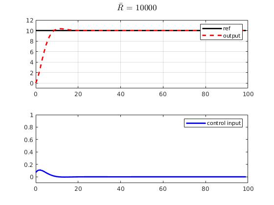
R_bar = 10000*eye(Nc,Nc);
for k = 1 : N_sim;
DeltaU = inv(Phi'*Phi + R_bar)*(Phi_R*r(k)-Phi_F*xf);
deltau = DeltaU(1,1);
u = u+deltau
u1(k) = u;
y1(k) = y;
xm_old = xm;
xm=Ad*xm+Bd*u
y = Cd*xm;
xf = [xm-xm_old;y];
end
k = 0:(N_sim-1);
figure
subplot(211)
plot(k,r,'k','LineWidth', 2);
hold on
plot(k,y1,'r--','LineWidth', 2);
grid on;
legend('ref', 'output');
ylim([-1 12]);
subplot(212)
plot(k,u1,'b','LineWidth', 2);
legend('control input');
ylim([-0.1 1])
%mpcgain.m
function [Phi, Phi_F, Phi_R, Ae, Be, Ce] = mpcgain(Ad, Bd, Cd, Nc, Np);

    %Ae, Be, Ce = Augmented Discrete-time model of Ad,Bd,Cd matrix
    %Ad, Bd, Cd is from c2dm of A, B, C

    %Continuous to discrete time model conversion example
%     A = [0 1 0; 3 0 1; 0 1 0];
%     B = [1; 1; 3];
%     C = [0 1 0];
%     D = zeros(1,1);
%     dt = 1;
%     [Ad, Bd, Cd, Dd] = c2dm(A,B,C,D,dt);

    %discrete to autmented discrete time model conversion
    % Ae = [ Ad 0; CdAd 1]
    % Be = [ Bd; CdBd]
    % Ce = [ 0 0 ... 0 (# of states)   1 1 ... 1 (# of outputs) ]
    [N_outputs, N_states] = size(Cd);
    [N_states, N_inputs] = size(Bd);
    Ae = eye(N_states+N_outputs, N_states+N_outputs);
    Ae(1:N_states, 1:N_states) = Ad;
    Ae(N_states+1:N_states+N_outputs, 1:N_states) = Cd*Ad;
    Be = zeros(N_states+N_outputs, N_inputs);
    Be(1:N_states,:) = Bd;
    Be(N_states+1:N_states+N_outputs,:) = Cd*Bd;
    Ce = zeros(N_outputs, N_states+N_outputs);
    Ce(:, N_states+1:N_states+N_outputs) = eye(N_outputs, N_outputs);

    h(1, :) = Ce;
    F(1, :) = Ce*Ae;

    for k = 2: Np
        h(k,:) = h(k-1, :)*Ae;
        F(k,:) = F(k-1,:)*Ae;
    end

    v = h*Be;
    Phi = zeros(Np,Nc);
    Phi(:,1) = v; % first column of Phi
    for i = 2 : Nc
        Phi(:,i) = [zeros(i-1,1); v(1:Np-i+1,1)];
%       Phi = Toeplitz (diagonal-constant) matrix
    end

    Rs = ones(Np,1);
    Phi_F = Phi'*F;
    Phi_R = Phi'*Rs;
end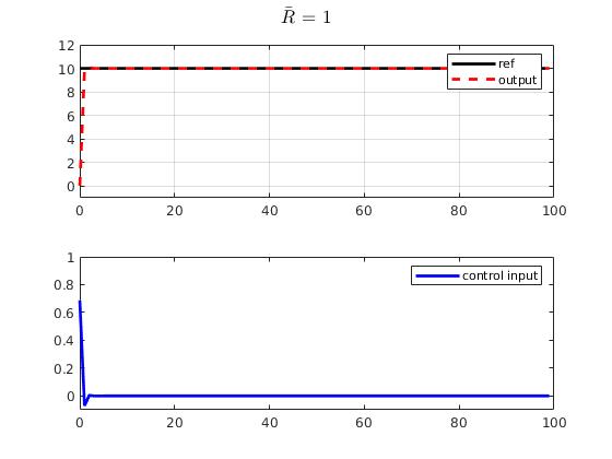
'Mathamatics > Control Theory' 카테고리의 다른 글
| ACADO Toolkit 이란? 1. Code Generation 방법 (0) | 2022.03.03 |
|---|---|
| MPC 란? (Model Predictive Control) 7. Multi-rotor system Model (0) | 2022.01.12 |
| MPC 란? (Model Predictive Control) 5. Controller Design (0) | 2022.01.11 |
| MPC 란? (Model Predictive Control) 4. Optimal control (1) | 2022.01.10 |
| MPC 란? (Model Predictive Control) 3. Prediction of state and output (0) | 2022.01.04 |

댓글